Bounding the largest eigenvalue of the random features gram matrix
I – Introduction
Consider a two-layer neural network on $d$-dimensional inputs, $k$ hidden neurons, activation function $\sigma:\mathbb R \to \mathbb R$, and one scalar output. Let the weights of each each hidden neuron $w_1,\ldots,w_k$ be sampled independently and uniformly from the unit-sphere in $\mathbb R^d$, and collected into a $k \times d$ random matrix $W$. Consider a sample of $n$ data points $x_1,\ldots,x_n$ independent of one another and of the weights matrix $W$, sampled independently and uniforml on the same sphere, and collected into an $n \times d$ random matrix $X$. Form the random $n \times k$ matrix $Z$ with entries $z_{aj} := \sigma(x_a^\top w_j)$, for some $1$-homogeneous continuous function $\sigma:\mathbb R \to \mathbb R$.
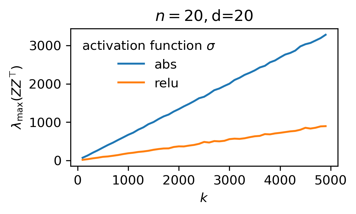
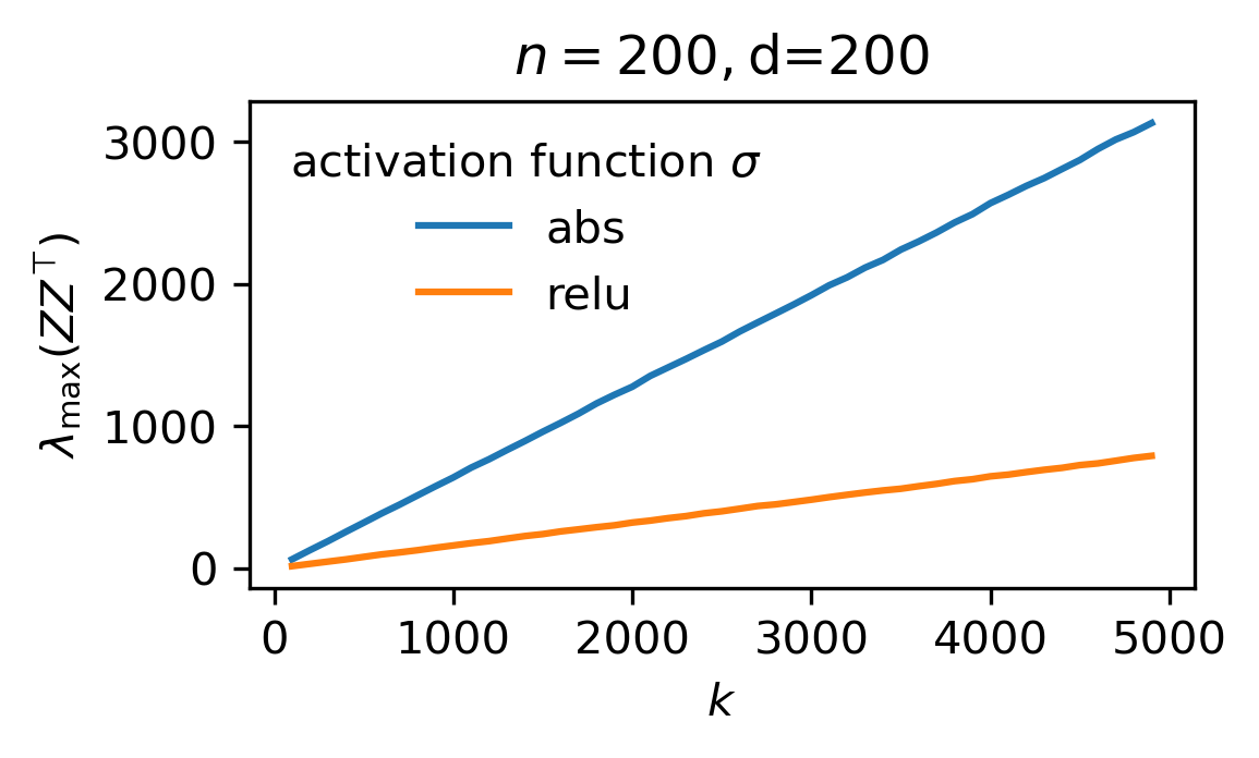
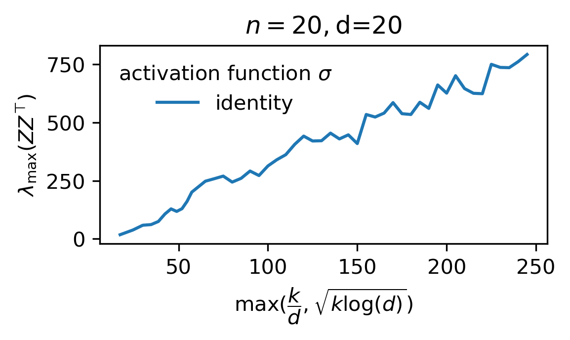
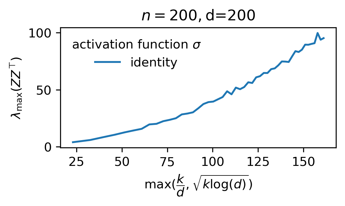
Goal. In this post, we are interested good probabilitistic upper-bounds on the largest eigenvalue of the $n \times n$ gram matrix $ZZ^\top$.
Now, we may write $ZZ^\top = \sum_{j=1}^k G_j$, where $G_j := \sigma(Xw_j) \otimes \sigma(Xw_j) \in \mathbb R^{n \times n}$, where $\sigma(Xw_j) := (\sigma(x_1^\top w_j),\ldots,\sigma(x_n^\top w_j)) \in \mathbb R^n$. Set $\overline{G}_j := G_j - \mathbb E_W[G_j]$. Note that thedue to $1$-homogeneity of the activaiton function $\sigma$, it is a direct consequence of Lemma 2.2.2 of Buchweitz (2016) that the $(a,b)$ entry of $\mathbb E[G_j]$ is given by
\[(\mathbb E[G_j])_{a,b} = \mathbb E_{w_j}[\sigma(x_a^\top w_j)\sigma(x_b^\top w_j)] = \frac{1}{d}\phi(x_a^\top x_b), \tag{*}\]for some $\phi:\mathbb R \to \mathbb R$ which is continuous on $(-1, 1]$ which is independent of $n$, $d$, and $k$. In particular the matrix $\mathbb E_{w_j} [G_j]$ is independent of the index $j \in [k]$. We will prove the following result
Main claim. Let $\Phi := (1/k)ZZ^\top$ and $\overline{\Phi} := \mathbb E_W[\Phi]$. For sufficiently large $n$, $d$, and $k$ such that $n=\mathcal O(d)$ and $k \gg \log d$, the following hold w.p $1-d^{-\Omega(1)}$ over $X$ and $W$.
- Concentration of entier eigenspectrum of normalized gram matrix: \(\|\Phi-\overline{\Phi}\|_{op} \le \sqrt{\dfrac{\log d}{k}}.\)
- Upper-bound on largest eigenvalue: \(\lambda_{\max}(\Phi) \le \begin{cases}\mathcal O(\max(\sqrt{\dfrac{\log d}{k}},\dfrac{1}{d})),&\mbox{ if }\phi\text{ is }\mathcal C^3\text{ at }0\text{ and }\phi(0) = 0,\\ \mathcal O(1),&\mbox{else.}\end{cases}\)


II – Proof (of main claim)
The proof is subdivided into sevral pieces, for the reader’s (and the writer’s!) convenience.
(1) Uniform upper-bound for spectral norm of the individual $G_j$’s. Standard RMT (see references at the end of this post) tells us that except on an event $\mathcal E$ which occurs w.p $1-e^{-\Omega(1)}$ or less, one has
\[\|X\|_{op} = \mathcal O(1)\text{ w.p }1-e^{-\Omega(d)}. \tag{2}\]Now, \(\|\overline{G}_j\|_{op} \le \|G_j\|_{op} + \|\mathbb E_{w_j}[G_j]\|_{op}\), and conditioned on the compliment $\mathcal E’$ of the event $\mathcal E$, one can bound \(\begin{split} \|G_j\|_{op} = \|\sigma(Xw_j)\|^2 &\le \sum_{a=1}^n (x_a^\top w_j)^2 = \|Xw_j\|^2 \le \|X\|_{op}^2 = \mathcal O(1). \end{split}\)
On the other hand, \(\|\mathbb E_{w_j}[G_j]\|_{op} = (1/d)\|\phi(XX^\top)\|_{op} = \mathcal O(n/d)=\mathcal O(1)\). Combining with the previous inequality gives \(\|\overline{G}_j\|_{op} = \mathcal O(1)\).
(2) Upper-bound for pseudo-variance. For simplicity, let $\phi_{ab} := \phi(x_a^\top x_b)$ and recall from (*) that $\mathbb E_{w_j}[z_{aj}z_{bj}] = (1/d)\phi_{ab}$. The $(a,b)$ entry of $\mathbb E_{w_j}[\overline{G_j}^2]$ writes
\[\begin{split} \mathbb E_{w_j}[(\overline{G_j}^2)_{a,b}] &= \sum_{c=1}^n \mathbb E_{w_j}[(\sigma(x_a^\top w_j)\sigma(x_c^\top w_j)-\frac{\phi_{ac}}{d})(\sigma(x_b^\top w_j)\sigma(x_c^\top w_j)-\frac{\phi_{bc}}{d})]\\ &= \sum_{c=1}^n \mathbb E_{w_j}[z_{aj}z_{bj} z_{cj}^2-z_{aj}z_{cj}\frac{\phi_{bc}}{d}-z_{bj}z_{cj}\frac{\phi_{ac}}{d}+\frac{\phi_{ac}\phi_{bc}}{d^2}]\\ &= \sum_{c=1}^n \mathbb E_{w_j}[z_{aj}z_{bj}z_{cj}^2] - \frac{\phi_{ac}\phi_{bc}}{d^2} = \sum_{c=1}^n \mathbb E_{w_j}[z_{aj}z_{bj}z_{cj}^2] - \mathcal O(\frac{n}{d^2}). \end{split} \tag{3}\]Thus, \(|\mathbb E_{w_j}[(\overline{G_j}^2)_{a,b}]| \le \mathcal O(1/d) + \sum_c \mathbb E_{w_j}[|z_{aj}z_{bj}|z_{cj}^2] \le \mathcal O(1/d) + \mathbb E_{w_j}[|z_{aj}z_{bj}|\sum_{c=1}^n z_{cj}^2]\). By Cauchy-Schwarz inequality, we have
\[(\mathbb E_{w_j}[|z_{aj}z_{bj}|\sum_{c=1}^n z_{cj}^2])^2 \le \mathbb E_{w_j}[z_{aj}^2 z_{bj}^2]\mathbb E_{w_j}[(\sum_{c=1}^n z_{cj}^2)^2].\]We bound each factor on the rightmost side like so:
- \(\mathbb E_{w_j}(\sum_{c=1}^n z_{cj}^2)^2 \le \mathbb E_{w_j}[(\sum_{c=1}^n (x_c^\top w_j)^2)^2] = \mathbb E_{w_j}\|Xw_j\|^4 \le \|X\|^4_{op} = \mathcal O(1)\) on the event $\mathcal E’$, and
- \(\mathbb E_{w_j}[z_{aj}^2z_{bj}^2] \le \|\phi\|_\infty ^2 \mathbb E_{w_j}[(x_a^\top w_j)^2(x_b^\top w_j)^2] = \|\phi\|_\infty^2\dfrac{(x_a^\top x_b)^2}{d(d+2)} \le \mathcal O(\dfrac{1}{d^2})\).
Combining with (3) gives \(\sup_{a,b \in [n]}|\mathbb E_{w_j}[(\overline{G_j}^2)_{a,b}]| \le \mathcal O(1/d)\) on the event $\mathcal E’$, and so \(v(ZZ^\top):= \sum_{j=1}^k \|\mathbb E_{w_j}[(\overline{G_j}^2)\|_{op} \le k \sup_{j=1}^k \|\mathbb E_{w_j}[\overline{G_j}^2]|\|_{op} \le k \cdot \mathcal O(n/d) = \mathcal O(k)\) on the same event.
(3) Matrix Bernstein inequality. By the matrix Bernstein inequality (see Tropp 2015), we obtain that conditioned on $\mathcal E’$, it holds with probability $1-\delta$ for $\delta = d^{-c}$ that,
\[\begin{split} \|\frac{1}{k}ZZ^\top - \mathbb E_{w_1}[G_1]\|_{op} &\le \sqrt{\frac{1}{k^2}v(ZZ^\top)\log d} + \mathcal O(\frac{1}{k}\log d)\\ &\lesssim \sqrt{\frac{1}{k}\log d} + \frac{1}{k}\log d \lesssim \sqrt{\frac{\log d}{k}}. \end{split} \tag{4}\]This proves the first part of the claim upon recalling that the “bad” event $\mathcal E$ only occurs with probability at most $d^{-\Omega(1)}$.
For the second part thanks to Proposition A.2 of Liang and Rakhlin (2018), we observe that
\[\|\mathbb E_{w_1}[G_1]\|_{op} = \dfrac{1}{d}\|\phi(XX^\top)\|_{op} \le \begin{cases} \dfrac{1}{d}\mathcal O(1)=\mathcal O(\dfrac{1}{d}),&\mbox{ if }\phi\text{ is "awful"},\\ \dfrac{1}{d}\mathcal O(n)=\mathcal O(\dfrac{n}{d})=\mathcal O(1),&\mbox{ else.} \end{cases}\]Thus, taking $t = (\log d)^c$ in (4) for an appropriate $c>0$, one gets the result, after recalling that $\mathcal E$ occurs w.p at most $d^{-\Omega(1)}$, the claim follows $\quad\quad\Box$.
III – References
- Introduction to the non-asymptotic analysis of random matrices, by Roman Vershynin.
- Topics in random matrix theory, by Terence Tao.
- Recent developments in non-asymptotic theory of random matrices, by Mark Rudelson.
- An Introduction to Matrix Concentration Inequalities, by Joel Tropp (2015).
- Concentration of functions beyond lévy’s inequality, by Erez Buchweitz (2016).
- Just Interpolate: Kernel “Ridgeless” Regression Can Generalize, Liang and Rakhlin (2018).