Variational auto-encoder for "Frey faces" using keras
In this post, I’ll demo variational auto-encoders [Kingma et al. 2014] on the “Frey faces” dataset, using the keras deep-learning Python library.
Some formal preliminaries
A well-known thermodynamic variational bound on surprise goes as follows:
\begin{equation} \begin{split} -\log p_G(x) = F_G(x) = F^R_G(x) - D_{KL}(p_R(.|x)||P_G(.|x)) \le F^R_G(x), \end{split} \end{equation} where
- $x$: Examplar datavector (visible layer).
- $z$: Hidden / latent variable (these are the ‘causes’ of the datavectors).
- $G$: Generative model, with density $z \sim p_G(.|x)$, parametrized by a tensor of weights $W^G$ (we’ll use a neural network)
- $R$: Recognition model, with density $z \sim p_R(.|x)$, parametrized by a tensor of weights $W^R$ (we’ill use a NN).
-
$D_{KL}(q||p)$ is the Kullback-Leibler divergence between probability densities $p$ and $q$, defined by \begin{equation} D_{KL}(q||p) := \sum_{z}q(z)\log(q(z)/p(z)) \end{equation}
- $F_G(x)$: Helmhost free-energy f a fictive thermodynamic system with macrostate energy levels $(E_G(z,x))_z$ with $E_G(z,x) := -\log(p_G(z,x))$, and partition function $p_G(x)$.
- $F^R_G(x)$ is the variational Helmholtz free-energy from $G$ to $R$, defined by \begin{equation} F_G^R(x) := \langle -\log(p_G(., x)) \rangle_{P_R(.|x)} - \mathcal H(P_R(.|x)), \end{equation} with \begin{equation} \mathcal H(p_R(.|x)) := -\sum_{z}p_R(z|x))\log(p_R(z|x)), \end{equation} the entropy of $p_R(.|x)$.
Problem: How do we sample from the recognition density $p_R(.|x)$ in such a way that the sampling process is differentiable w.r.t the weights of the recognition network $ W^R$ ?
Solution: The reparametrization trick!
The solution proposed in [Kingma et al. 2014] is to use a reparametrization trick:
- Choose $\epsilon \sim p_{\text{noise}}$ (noise distribution, independent of $W^R$! )
-
Set $z = g(W^{R}, x, \epsilon)$, where $g$ is an appropriate class $\mathcal C^1$ function.
$ \implies $ a sample $z \sim p_R(.|x)$, from the correct posterior
The code
Dependencies: We’ll need the following python libraries to get things running:
- Numpy / Scipy (install everything via anaconda)
- keras
- Theano or Tensforflow (as backend for Keras)
A bit of setup
import numpy as np
import matplotlib.pyplot as plt

# configure matplotlib
%matplotlib inline
plt.rcParams['figure.figsize'] = (13.5, 13.5) # set default size of plots
plt.rcParams['image.interpolation'] = 'nearest'
plt.rcParams['image.cmap'] = 'gray'

# for auto-reloading external modules
# see http://stackoverflow.com/questions/1907993/autoreload-of-modules-in-ipython
%load_ext autoreload
%autoreload 2
Now, let’s load the dataset
import os
from urllib2 import urlopen, URLError, HTTPError
from scipy.io import loadmat


def fetch_file(url):
    """Downloads a file from a URL.
    """
    try:
        f = urlopen(url)
        print "Downloading data file " + url + " ..."

        # Open our local file for writing
        with open(os.path.basename(url), "wb") as local_file:
            local_file.write(f.read())
        print "Done."

    #handle errors
    except HTTPError, e:
        print "HTTP Error:", e.code, url
    except URLError, e:
        print "URL Error:", e.reason, url

url =  "http://www.cs.nyu.edu/~roweis/data/frey_rawface.mat"
data_filename = os.path.basename(url)
if not os.path.exists(data_filename):
    fetch_file(url)
else:
    print "Data file %s exists." % data_filename

# reshape data for later convenience
img_rows, img_cols = 28, 20
ff = loadmat(data_filename, squeeze_me=True, struct_as_record=False)
ff = ff["ff"].T.reshape((-1, img_rows, img_cols))
… and split data into train / validation folds
np.random.seed(42)
n_pixels = img_rows * img_cols
X_train = ff[:1800]
X_val = ff[1800:1900]
X_train = X_train.astype('float32') / 255.
X_val = X_val.astype('float32') / 255.
X_train = X_train.reshape((len(X_train), n_pixels))
X_val = X_val.reshape((len(X_val), n_pixels))
Visualize some examples from the dataset
def show_examples(data, n=None, n_cols=20, thumbnail_cb=None):
    if n is None:
        n = len(data)
    n_rows = int(np.ceil(n / float(n_cols)))
    figure = np.zeros((img_rows * n_rows, img_cols * n_cols))
    for k, x in enumerate(data[:n]):
        r = k // n_cols
        c = k % n_cols
        figure[r * img_rows: (r + 1) * img_rows,
               c * img_cols: (c + 1) * img_cols] = x
        if thumbnail_cb is not None:
            thumbnail_cb(locals())

    plt.figure(figsize=(12, 10))
    plt.imshow(figure)
    plt.axis("off")
    plt.tight_layout()
show_examples(ff, n=200, n_cols=25)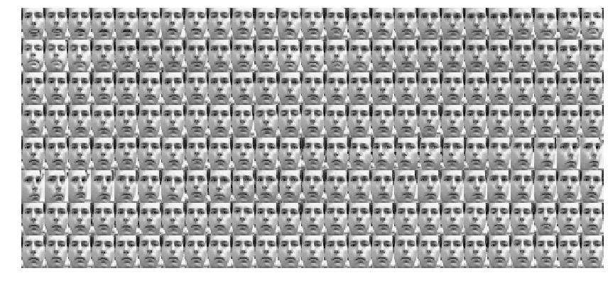
Build forward model (encoding)
from keras import backend
from keras.layers import Input, Dense, Lambda
from keras.models import Model
from keras.objectives import binary_crossentropy

intermediate_dim = 256
latent_dim = 2
batch_size = 100
nb_epoch = 100
noise_std = .01
x = Input(shape=(n_pixels,))
h = Dense(intermediate_dim, activation="relu")(x)
z_mean = Dense(latent_dim)(h)
z_log_var = Dense(latent_dim)(h)
Sample from latent space
def sampling(args):
    z_mean, z_log_var = args
    epsilon = backend.random_normal(shape=(batch_size, latent_dim), mean=0., std=noise_std)
    epsilon *= backend.exp(.5 * z_log_var)
    epsilon += z_mean
    return epsilon
z = Lambda(sampling, output_shape=(latent_dim,))([z_mean, z_log_var])
Build backward model (decoding)
decoder_h1 = Dense(intermediate_dim, activation="relu")
decoder_h2 = Dense(n_pixels, activation="sigmoid")
z_decoded = decoder_h1(z)
x_decoded = decoder_h2(z_decoded)
Build the autoencder
vae = Model(input=x, output=x_decoded)
from keras.utils import visualize_util as vizu
vizu.plot(vae, "ff.png", show_layer_names=False, show_shapes=True)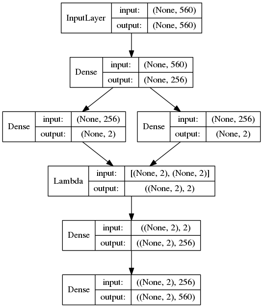
# Objective function minimized by autoencoder
def vae_objective(x, x_decoded):
    loss = binary_crossentropy(x, x_decoded)
    kl_regu = -.5 * backend.sum(1. + z_log_var - backend.square(
        z_mean) - backend.exp(z_log_var), axis=-1)
    return loss + kl_regu
# Compile the autoencoder computation graph
vae.compile(optimizer="adam", loss=vae_objective)Train the autoencoder (or reload a previously trained one)
import os
weights_file = "ff_%d_latent.hdf5" % latent_dim
if os.path.isfile(weights_file):
    vae.load_weights(weights_file)
else:
    from keras.callbacks import History
    hist_cb = History()
    vae.fit(X_train, X_train, shuffle=True, nb_epoch=nb_epoch, batch_size=batch_size,
            callbacks=[hist_cb], validation_data=(X_val, X_val))
    vae.save_weights(weights_file)

    # plot convergence curves to show off
    plt.plot(hist_cb.history["loss"], label="training")
    plt.plot(hist_cb.history["val_loss"], label="validation")
    plt.grid("on")
    plt.xlabel("epoch")
    plt.ylabel("loss")
    plt.legend(loc="best")
Separate encoder from input to latent space
encoder = Model(input=x, output=z_mean)Generator from latent to input space
decoder_input = Input(shape=(latent_dim,))
h_decoded = decoder_h1(decoder_input)
x_decoded = decoder_h2(h_decoded)
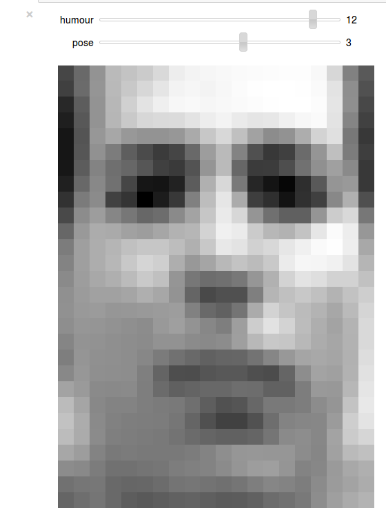
generator = Model(input=decoder_input, output=x_decoded)Display a 2D manifold of the faces. In this example we found that the each dimension of the hidden variable z was encoding for socially meaningful things like humour / expression & pose
from ipywidgets import FloatSlider, interact

we will sample points within given standard deviations
humour = FloatSlider(min=-15, max=15, step=3, value=0)
pose = FloatSlider(min=-15, max=15, step=3, value=0)

@interact(pose=pose, humour=humour)
def do_thumb(humour, pose):
    z_sample = np.array([[humour, pose]]) * noise_std
    x_decoded = generator.predict(z_sample)
    face = x_decoded[0].reshape(img_rows, img_cols)
    plt.figure(figsize=(11.5, 11.5))
    ax = plt.subplot(111)
    ax.imshow(face)
    plt.axis("off")