Learning brain regions from large-scale online structured sparse DL
In our NIPS 2016, paper, we propose a multivariate online dictionary-learning method for obtaining decompositions of brain images with structured and sparse components (aka atoms). Sparsity is to be understood in the usual sense: the dictionary atoms are constrained to contain mostly zeros. This is imposed via an L1-norm constraint. By “structured”, we mean that the atoms are piece-wise smooth and compact, thus making up blobs, as opposed to scattered patterns of activation. We propose to use a Sobolev (Laplacian) penalty to impose this type of structure. Combining the two penalties, we obtain decompositions that properly delineate brain structures from functional images. This non-trivially extends the online dictionary-learning work of Mairal et al. (2010), at the price of only a factor of 2 or 3 on the overall running time. Just like the Mairal et al. (2010) reference method, the online nature of our proposed algorithm allows it to scale to arbitrarily sized datasets. Experiments on brain data show that our proposed method extracts structured and denoised dictionaries that are more intepretable and better capture inter-subject variability in small medium, and large-scale regimes alike, compared to state-of-the-art models.
In this blog post, I’ll throw some light on the main ideas.
\[\def\EE{\mathbb E} \def\RR{\mathbb R} \def\PP{\mathbb P} \def\A{\mathbf A} \def\D{\mathbf D} \def\M{\mathbf M} \def\X{\mathbf X} \def\b{\mathbf b} \def\a{\mathbf a} \def\d{\mathbf d} \def\x{\mathbf x} \def\balpha{\boldsymbol{\alpha}} \def\argmin{\text{argmin}} \def\Id{\mathbf I} \def\1{\mathbf 1} \def\x{\mathbf x} \def\y{\mathbf y} \def\u{\mathbf u} \def\v{\mathbf v} \def\X{\mathbf X} \def\Y{\mathbf Y} \def\Z{\mathbf Z} \def\A{\mathbf A} \def\B{\mathbf B} \def\U{\mathbf U} \def\V{\mathbf V}\]The problem
Consider a stack $\X \in \mathbb R^{n \times p}$ of $n$ subject-level brain images $\X_1,\X_2,\ldots,\X_n$ each of shape $n_1 \times n_2 \times n_3$, over a mask $\mathcal M \subseteq \mathbb R^3$ containing $p$ voxels. Each image can thus be seen as $p$-dimensional row-vector. These images $\X_i$ could be images of fMRI activity patterns like statistical parametric maps of brain activation, raw pre-registered (into a common coordinate space) fMRI time-series, PET images, etc. We would like to decompose these images as a product of $k \le \min(n, p)$ component maps (aka latent factors or dictionary atoms) $\V^1, \ldots, \V^k \in \mathbb{R}^{p \times 1}$ and modulation coefficients $\U_1, \ldots, \U_n \in \mathbb R^{k \times 1}$ called \textit{codes} (one $k$-dimensional code per sample point), i.e \begin{eqnarray} \X_i \approx \V \U_i, \text{ for } i=1,2,\ldots,n \end{eqnarray} where $\V := [\V^1|\ldots|\V^k] \in \mathbb{R}^{p \times k}$, an unknown dictionary to be estimated. Typically, $p \sim 10^{5}$ – $10^{6}$ (in full-brain high-resolution fMRI) and $n \sim 10^{2}$ – $10^{5}$ (for example, in considering all the 500 subjects and all the about 15 –20 functional tasks of the Human Connectome Project dataset. Our work handles the extreme case where both $n$ and $p$ are large (massive-data setting).
It is reasonable then to only consider under-complete dictionaries: $k \le \min(n, p)$. Typically, we use $k \sim 50$ or $100$ components.
It should be noted that online optimization is not only crucial in the case where $n / p$ is big; it is relevant whenever $n$ is large, leading to prohibitive memory issues irrespective of how big or small $p$ is.
Our model: Smooth Sparse Online Dictionary-Learning (Smooth-SODL)
We’d want the component maps (aka dictionary atoms) $\V^j$ to be sparse and spatially smooth. A principled way to achieve such a goal is to impose a boundedness constraint on $\ell_1$-like norms of these maps to achieve sparsity and simultaneously impose smoothness by penalizing their Laplacian. Thus, we propose the following penalized dictionary-learning model
\[\begin{aligned} &\min_{\V \in \mathbb R^{p \times k}}\left(\lim_{n \rightarrow \infty}\frac{1}{n}\sum_{i=1}^n\min_{\U_i \in \mathbb R^{k}}\frac{1}{2} \|\X_i-\V\U_i\|_2^2 + \frac{1}{2}\alpha\|\U_i\|_2^2\right) + \gamma\sum_{j=1}^k\Omega_{\text{Lap}}(\V^j).\\ &\text{subject to }\V^1,\ldots,\V^k \in \mathcal C \end{aligned}\]The ingredients in the model can be broken down as follows:
- The constraint set $\mathcal C$ is a sparsity-inducing compact simple (mainly in the sense that the Euclidean projection onto $\mathcal C$ should be easy to compute) convex subset of $\mathbb R^p$ like an $\ell_1$-ball $\mathbb B_{p,\ell_1}(\tau)$ or a simplex $\mathcal S_p(\tau)$, defined respectively as
and $\mathcal S_p(\tau) := \mathbb B_{p,\ell_1}(\tau) \cap \mathbb R_+^p.$ Other choices (e.g ElasticNet ball) are of course possible. The radius parameter $\tau > 0$ controls the amount of sparsity: smaller values lead to sparser atoms.
-
Each of the terms $\max_{\U_i \in \mathbb R^k}\dfrac{1}{2}||\X_i-\V\U_i||_2^2$ measures how well the current dictionary $\V$ explains data $\X_i$ from subject $i$. onstruction error for subject $i$. Both the $\U$ and $\V$ matrices are parameters to be estimated. The Ridge penalty term $\phi(\U_i) \equiv \frac{1}{2}\alpha||\U_i||_2^2$ on the codes amounts to assuming that the energy of the decomposition is spread across the different samples. In the context of a specific neuro-imaging problem, if there are good grounds to assume that each sample / subject should be sparsely encoded across only a few atoms of the dictionary, then we can use the $\ell_1$ penalty $\phi(\U_i) := \alpha||\U_i||_1$ as in [Mairal 2010]. We note that in contrast to the $\ell_1$ penalty, the Ridge leads to stable codes. The parameter $\alpha > 0$ controls the amount of penalization on the codes.
-
Finally, $\Omega_{\text{Lap}}$ is the 3D Laplacian regularization functional defined by
where $\nabla_x$ being the discrete spatial gradient operator along the $x$-axis (N.B.: the input vector $\v$ is unmasked into a 3d image according to the afore-mentioned mask $\mathcal M$ before the image gradient is computed), etc., and $\Delta := \nabla^T\nabla$ is the $p$-by-$p$ matrix representing the discrete Laplacian operator. This penalty is meant to impose blobs. The regularization parameter $\gamma \ge 0$ controls how much regularization we impose on the atoms, compared to the reconstruction error.
The above formulation, which we dub Smooth Sparse Online Dictionary-Learning (Smooth-SODL) is inspired by, and generalizes the standard dictionary-learning framework of [Mairal 2010] –henceforth referred to as Sparse Online Dictionary-Learning (SODL); setting $\gamma = 0$, we recover SODL [Mairal 2010].
Estimating the model
The objective function in problem of the Smooth-SODL model above is separately convex and block-separable w.r.t each of $\U$ and $\V$ but is not jointly convex in $(\U,\V)$. Also, it is continuously differentiable on the constraint set, which is compact and convex. Thus by classical results (e.g [Bertsekas 1999]), the problem can be solved via Block-Coordinate Descent (BCD) [Mairal 2010]. Reasoning along the lines of [Jenatton 2010], we derive that the BCD iterates are as given in an algorithm presented further below. A crucial advantage of using a BCD scheme is that it is parameter free: there is not step size to tune.
The Algorithm
The resulting online algorithm is adapted from [Mairal 2010].
- Require
- Regularization parameters $\alpha, \gamma > 0$.
- Initial dictionary $\V \in \mathbb R^{p \times k}$.
- Number of passes / iterations $T$ on the data.
- Set $\A_0 \leftarrow 0 \in \mathbb R^{k \times k}$, $\B_0 \leftarrow 0 \in \mathbb R^{p \times k}$ \text (historical ``sufficient statistics’’)
- For $t = 1$ to $T$, do
- Empirically draw a sample point $\X_t$ at random.
- Code update: Ridge-regression (via SVD of current dictionary $\V$) \(\U_t \leftarrow \argmin_{\u \in \mathbb R^k}\frac{1}{2}\|\X_t - \V \u\|_2^2 + \frac{1}{2}\alpha\|\u\|_2^2.\)
- Rank-1 updates: $\A_t \leftarrow \A_{t-1} + \U_t\U_t^T,\; \B_t \leftarrow \B_{t-1} + \X_t\U_t^T$
- BCD dictionary update: Compute update for dictionary $\V$ using the algorithm below.
Updating the dictionary $\V$
For updating the dictionary atoms $\V^j$ , we proposed the following algorithm:
- Require $\V = [\V^1|\ldots|\V^k] \in \mathbb{R}^{p \times k}$ (input dictionary).
- Set $\A = [\A^1|\ldots|\A^k] \in \mathbb R^{k \times k}$, $\B_t = [\B_t^1|\ldots|\B_t^k] \in \mathbb R^{p \times k}$ (history)
- While stopping criteria not met, do
- For $j = 1$ to $r$, do
- Fix the code $\U$ and all atoms $k \ne j$ of the dictionary $\V$ and then update $\V^j$ as follows \(\begin{aligned} \V^j &\leftarrow \argmin_{\v \in \mathcal C}F_{\gamma (\A_t[j,j]/t)^{-1}}(\v, \V^j + \A_t[j,j]^{-1}(\B_t^j - \V\A_j)), \end{aligned}\) where \(F_{\tilde{\gamma}}(\v,\a) \equiv \frac{1}{2}\|\v - \a\|_2^2 + \tilde{\gamma}\Omega_{\text{Lap}}(\v) = \frac{1}{2}\|\v - \a\|_2^2 + \frac{1}{2}\tilde{\gamma}\v^T\Delta\v.\)
- For $j = 1$ to $r$, do
Details and proofs are given in the NIPS paper. Parameter selection is also discussed there.
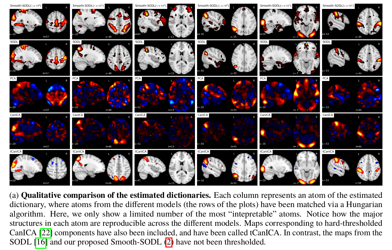
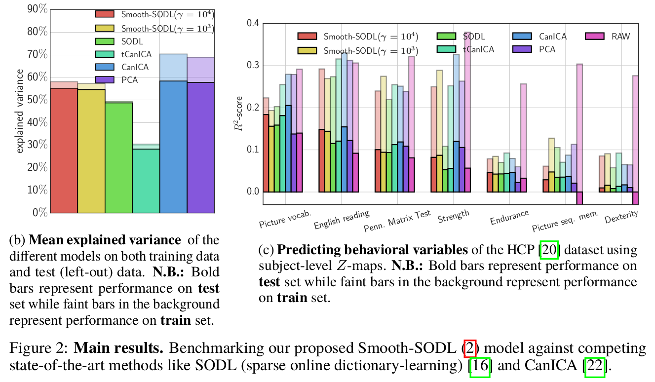
Results

Concluding remarks
To extract structured functionally discriminating patterns from massive brain data (i.e data-driven atlases), we have extended the online dictionary-learning framework first developed in [Mairal 2010], to learn structured regions representative of brain organization. To this end, we have successfully augmented [Mairal 2010] with a Laplacian prior on the component maps, while conserving the low numerical complexity of the latter. Through experiments, we have shown that the resultant model –Smooth-SODL model – extracts structured and denoised dictionaries that are more intepretable and better capture inter-subject variability in small medium, and large-scale regimes alike, compared to state-of-the-art models. We believe such online multivariate online methods shall become the de facto way do dimensionality reduction and ROI extraction in future.